AAPG '98 Annual Convention, Advances in Geostatistics

AAPG '98 Annual Convention, Advances in Geostatistics, Salt Lake City, Utah, May 17-20, 1998.

PDF File: Pre-formatted paper as presented in proceedings.

Classes vs. Thresholds: A Modification to Traditional Indicator Simulation

William L. Wingle and Eileen P. Poeter, Colorado School of Mines, Department of Geology and Geological Engineering

Summary

When using traditional discrete multiple indicator conditional simulation, semivariogram models are based on the spatial variance of data above and below selected thresholds (cut-offs). There are two problems though; 1) the spatial distribution of a threshold can be difficult to conceptualize, and 2) ordering of the indicators may influence the results, unfortunately to change the arbitrary order, to test sensitivity, involves substantial effort. If the conditional simulations instead are based on the indicators themselves (classes), rather than the thresholds separating the indicators, then the spatial statistics are more intuitive, and reordering the indicators becomes a trivial endeavor. When class indicators are used, the indicator order can be switched at any time without recalculating the semivariograms. If thresholds are used, and the ordering is changed, all the semivariograms must be recalculated. A final advantage of using the class approach is that semivariograms calculated from transition probabilities go directly into the simulation. Despite significant differences in the methods, the simulation results are nearly identical, for cases where ordering does not cause differences when using the threshold approach. Given the consistency resulting from the class approach and its ease of use, this approach is preferred.

Introduction

In traditional Multiple Indicator Conditional Simulation (MICS), the kriged model results are based on semivariograms describing the spatial distribution of the thresholds between indicators. The affect of the order of the indicators on the resulting realizations is rarely evaluated even though the numerical order is arbitrary. For traditional simulation, the estimated indicator at a location is based on the probability that the location is below each threshold (the number of thresholds equals the number of indicators minus one). A more intuitive approach is based on calculating the probability of occurrence of each individual indicator. This paper presents a technique which uses semivariogram models based on individual indicators (classes), as opposed to the traditional threshold semivariograms which are based on the indicators below a cut-off versus the indicators above the cut-off.

These differences can be described mathematically as follows. Where the data set has been differentiated into a finite number of indicators, it is possible to define a random function (Z(x)) whose outcomes will have values in the range z_min to z_max. From the definition of the indicators, K thresholds can be defined (K + 1 equals the number of indicators) where:

(1)

The random variable Z(x) can then be transformed into an indicator random variable I(x:z_k) by:

(2)

The first moment of the indicator transform yields:

(3)

where E{I(x:z_k)} is the expectation of I(x:z_k), and P{Z(x) < z_k} and P{Z(x) > z_k} are the probabilities Z(x) is less than or greater than the threshold z_k. This equation is equivalent to the univariate cumulative distribution function (CDF) of Z(x). For classes, similar equations can be defined. Classes (c_i) are equivalent to the indicators defined using thresholds in equation 1, and are defined:

(4)

Once the classes are defined, the random variable Z(x) can be transformed into an indicator random variable I(x:z_k) by:

(5)

and the first moment of the indicator transform yields:

(6)

In this case, the univariate probability distribution function (PDF) is defined. By summing the PDF components, the univariate CDF is obtained.

Because the equations to define the class or threshold expectation are fundamentally the same, the class method generates realizations that are equally accurate to threshold realizations, but with three advantages. First, it is easier to conceptually relate the model semivariograms to the spatial distribution of the geologic units. When class semivariograms are calculated, the range reflects the average size of the units, whereas the threshold semivariograms represent the distribution of indicators above or below a threshold and these can be difficult to conceptually equate to units in complex geologic settings. The first and last class and threshold semivariograms will always be identical (they are based on equivalent indicator sets), however the intermediate semivariograms may vary substantially. The intuitive sense for the threshold semivariogram range decreases with an increasing number of indicators, while Class semivariogram ranges, still reflect the average size of the unit. The second advantage to using classes is that sensitivity to indicator ordering can be evaluated without developing additional semivariogram models. If thresholds are used, the full suite of threshold semivariogram models must be recalculated for each reordering. The final advantage is that semivariograms can be calculated for transition probabilities (Carle and Fogg, 1996). The class approach does have several disadvantages: 1) more order relation violations occur, though because of the techniques utilized with thresholds, some of these may simply not be visible, though present, 2) it is computationally more expensive (one additional kriging matrix must be solved per grid cell), and 3) it requires one additional semivariogram model definition. The last two items are only a concern, if ordering sensitivity is not evaluated. If sensitivity to ordering is a concern, preparation for the threshold method requires far more human effort and computer time to develop and analyze the additional semivariogram models.

Methods

To use classes, the threshold simulation process is modified at the data definition level, and in the evaluation of the kriged CDF.

Data Definition

To calculate a threshold indicator semivariogram, an individual threshold is selected. All values below the threshold are assigned a 1, and values above the threshold are assigned a 0. For class semivariograms, locations with sample values that are in the class being evaluated are set to 1, the remaining values are set to 0.

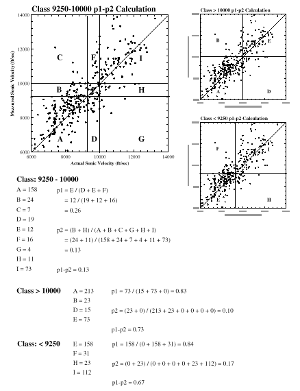
If imprecise soft data are used (data with non-negligible uncertainty), with associated misclassification probabilities, the following steps are required. First, the probability that the data correctly, or incorrectly, reflect the class is defined using misclassification probabilities (p₁ and p₂):

p₁: Given that the actual value is less than the threshold (in the class), p₁ is the probability that the measured value is less than the threshold (in the class).

p₂: Given that the actual value is not less than the threshold (not in class), p₂ is the probability that the measured value is less than the threshold (in the class).

These values are determined by comparing the soft data to co-located hard data using a training set. After p₁ and p₂ have been determined, the misclassification probabilities can be used for the same type of soft data, at locations where hard data are not present.

Using indicator thresholds, p₁ and p₂ are determined by measuring the ability of soft information to correctly classify the hard training set data above and below a specified threshold level. The misclassification probabilities are defined as:

(7)

(8)

In region A, points are correctly classified below the specified threshold, in C, they are correctly defined as above the threshold. In regions B and D, the soft data incorrectly classify the sample. Ideally p₁ is greater than p₂. For hard data p₁ = 1.0 and p₂ = 0.0. If the soft data are not correlated with the hard data p₁ = p₂ (NOTE: p₁ and p₂ are not expected to sum to 1.0). The difference between p₁ and p₂ indicates the quality of the soft data. When using indicator classes, rather than thresholds, the implications of p₁ and p₂ are the same, but calculation is more complex and p₂ tends to increase as the number of classes increase. A graphical representation for calculating p₁ and p₂ is shown for three classes in Figure 1. The misclassification probabilities are defined as:

(9)

(10)

In region E, points are correctly classified as being included in the specified class. In regions A, C, G, and I, they are correctly defined as being outside of the class. In regions B, D, F, and H, the soft data incorrectly classify the sample.

FIGURE 1: Graphical method of calculating p₁ and p₂ values for a specific class. Data from CSM Survey Field.

The p₁-p₂ misclassifications for the class and threshold approaches are identical for the first and last indicators, because the upper or lower bound is missing, and the class equations reduce to those for thresholds. For other classes and thresholds, p₁ and p₂ estimates vary significantly. For thresholds, the soft sample values need only be on the correct side of the cut-off for the threshold to correctly identify the hard data sample. Using classes, the soft data have both high and low cut-offs, therefore the soft data must precisely identify a location as a member (or not) of a hard data class (Figure 1). This is a more restrictive constraint and as a result, the class p₁-p₂ values are lower than those for threshold simulation. The quality of the soft data has not changed, it is just defined differently. What has changed is the ability of the algorithm to describe the imprecision.

Difference Between Prior Hard and Prior Soft Data CDF's for Class and Threshold Simulations

An additional and important difference between class and threshold simulation is the definition and treatment of the difference in the hard data and soft data prior probability distributions. Often, hard and soft data collection techniques suggest different percentages of each indicator occurring at the site. If the simulator uses thresholds, the correction term is based on:

| (% hard data < threshold) - (% soft data < threshold) |

If classes are used, the correction term is based on:

| (% hard data = class) - (% soft data = class) |

The difference is subtle, but important. For the threshold approach, if the probability of a single threshold varies significantly between the hard and soft data, the importance of the remaining thresholds can be under-valued. Reordering the indicators can alleviate some of this problem. For the class approach, the relative occurrence of each indicator is directly compared, therefore when one class has very different prior hard and prior soft probabilities, it does not seriously affect other class estimates, because the error is not cumulative.

Order Relation Violations

As with traditional threshold simulation, the class CDF for a particular grid location may not be monotonically increasing and may not sum to 1.0. These are order relation violations (ORV's). They can be caused by use of inconsistent semivariogram models for the different thresholds or classes, or by use of different prior probabilities and p₁-p₂ weights applied to soft data. Threshold and class methods manage ORV's differently, due to differences in how the CDF's are generated, and technical difficulties in reducing the threshold CDF to a PDF.

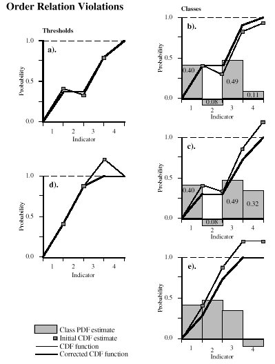
One type of ORV occurs when the CDF declines from one threshold to the next (Figure 2a). A CDF is a cumulative probability, so a declining CDF is an impossibility. It is not possible to determine which threshold causes the problem, therefore to remedy the situation, the average of the two probabilities is assigned to both thresholds. For classes, the equivalent problem is an individual class having a negative probability of occurrence (Figure 2b: indicator #2), which is also an impossibility. In this case though, it is reasonable to assign that class a zero probability of occurrence. There is no reason to distribute the error to another unrelated indicator.

FIGURE 2: For both the class and threshold approach, there are two basic types of order relation violations (ORV). a) An individual CDF probability is less than the CDF of a smaller threshold (the CDF is decreasing); this is equivalent to a class having a negative probability of occurence. This type of ORV is resolved for thresholds by averaging the two CDF's so that they are equal; for classes, a 0.0 probability of occurence is assigned to the PDF. b) When cumulative probabilities are greater than 1.0, the value is truncated to 1.0 for the threshold approach, while for the class approach, the probability for each class is proportionally rescaled, so that the CDF will sum to 1.0.

Another type of ORV occurs when the CDF sums to a value greater than, or less than 1.0. For thresholds, the last threshold CDF term is often less than 1.0 (Figure 2a), and it is assumed that the balance of the CDF is described by the final indicator. This may be true, but as shown in an equivalent class example, it is possible for the final indicator to account for significantly more (or less) than the remaining portion of the CDF (Figure 2c). With classes, the overestimate in the CDF is proportionally absorbed by each of the PDF components (PDFnew = PDFold / CDFfinal value). In this example, the threshold method would not have recognized that an ORV occurred and there would be no correction. The CDF may also exceed 1.0 (Figure 2d). Some threshold algorithms manage this problem by truncating the CDF to 1.0 for the affected threshold (and all following thresholds). This solution is not very satisfying, in part, because it implies the offending threshold level is fully responsible for the error, even though the CDF is a cumulative probability (i.e., an earlier threshold could be the cause of the problem), and because of this, it biases results to the lower order indicators. Classes again, manage this situation by distributing the error over all the PDF components (Figure 2e).

These techniques for managing class ORV's are less biased then the threshold method. This is fortunate, since the class method also produces more ORV's. However, these additional ORV's are basically ignored by the threshold approach (compare Figures 2a vs. 2c).

Conclusions

Class simulation has significant advantages over threshold simulation:

Class simulation is more intuitive.
Testing simulation sensitivity to indicator ordering is trivial to setup.
The last CDF value is calculated rather than implied.
Class simulation better identifies ORV's, and correctly adjusts the weights.
Hard and soft data prior probabilities differences tend to be smaller.
Semivariograms can be calculated from transition probabilities.

There are some disadvantages to using classes too:

Class simulation yields poorer p₁-p₂ estimates.
Class simulation requires one additional semivariogram model.
Class simulation is computationally more expensive.

The last two disadvantages, are insignificant if indicators are reordered to test model sensitivity.

Acknowledgments

We appreciate the United States Army Corps of Engineers, Waterways Experiment Station for supporting this research.

References

Alabert, F.G., 1987, Stochastic Imaging and Spatial Distributions Using Hard and Soft Information. Master's Thesis, Department of Applied Earth Sciences. Stanford, Stanford University.

Carle, S.F. and G.E. Fogg, 1996, ``Transition Probability-Based Indicator Geostatistics.'' Mathematical Geology, Vol. 28, No. 4, pp. 453-476.

Gómez-Hernández, J.J. and R.M. Srivastava, 1990, ``ISIM3D: An ANSI-C Three Dimensional Multiple Indicator Conditional Simulation Program.'' Computers in Geoscience, Vol. 16, No. 4, pp. 395-440.

Journel, A.G. and C.J. Huijbregts, 1978, Mining Geostatistics. London, Academic Press.